Decision Tree for Continuous Variable in R

Overview of Decision Tree in R

Decision Tree in R is a machine-learning algorithm that can be a classification or regression tree analysis. The decision tree can be represented by graphical representation as a tree with leaves and branches structure. The leaves are generally the data points and branches are the condition to make decisions for the class of data set. Decision trees in R are considered as supervised Machine learning models as possible outcomes of the decision points are well defined for the data set. It is also known as the CART model or Classification and Regression Trees. There is a popular R package known as rpart which is used to create the decision trees in R.

Decision tree in R

To work with a Decision tree in R or in layman terms it is necessary to work with big data sets and direct usage of built-in R packages makes the work easier. A decision tree is non- linear assumption model that uses a tree structure to classify the relationships. The Decision tree in R uses two types of variables: categorical variable (Yes or No) and continuous variables. The terminologies of the Decision Tree consisting of the root node (forms a class label), decision nodes(sub-nodes), terminal node (do not split further). The unique concept behind this machine learning approach is they classify the given data into classes that form yes or no flow (if-else approach) and represents the results in a tree structure. The algorithm used in the Decision Tree in R is the Gini Index, information gain, Entropy. There are different packages available to build a decision tree in R: rpart (recursive), party, random Forest, CART (classification and regression). It is quite easy to implement a Decision Tree in R.

For clear analysis, the tree is divided into groups: a training set and a test set. The following implementation uses a car dataset. This data set contains 1727 obs and 9 variables, with which classification tree is built. In this article lets tree a 'party 'package. The function creates () gives conditional trees with the plot function.

Implementation using R

The objective is to study a car data set to predict whether a car value is high/low and medium.

i. Preparing Data

Installing the packages and load libraries

This module reads the dataset as a complete data frame and the structure of the data is given as follows:

data<-car // Reading the data as a data frame
str(data) // Displaying the structure and the result shows the predictor values.

Output:

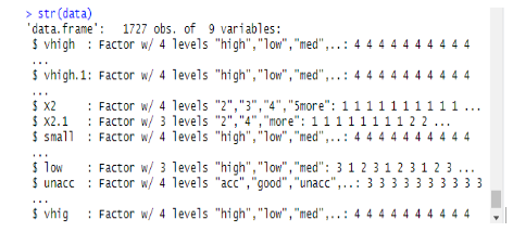
Determining Factordata$vhigh<-factor(data$vhigh)> View(car)
> data<-car

ii. Partition a data

Splitting up the data using training data sets. A decision tree is split into sub-nodes to have good accuracy. The complexity is determined by the size of the tree and the error rate. Here doing reproductivity and generating a number of rows.

set. Seed (1234)
dt<-sample (2, nrow(data), replace = TRUE, prob=c (0.8,0.2))
validate<-data[dt==2,]

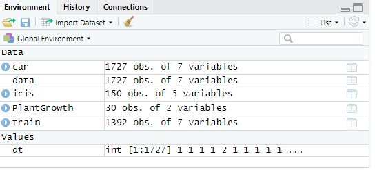
Fig: Showing data values

Next, making data value to 2

validate<-data[dt==2,]

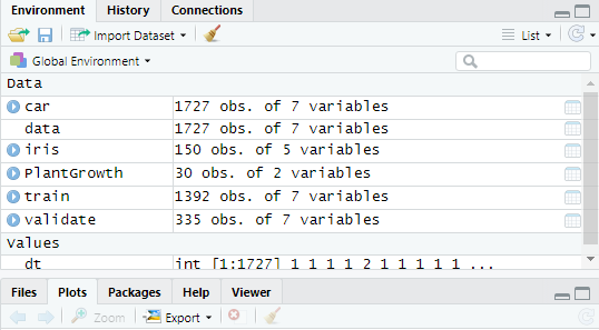
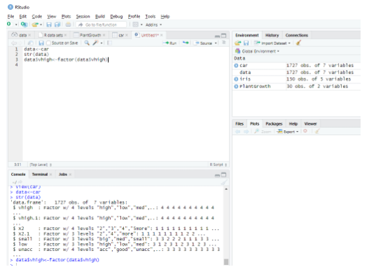
Fig: Displaying R console in R Studio

Creating a Decision Tree in R with the package party

• Click package-> install -> party. Here we have taken the first three inputs from the sample of 1727 observations on datasets. Creating a model to predict high, low, medium among the inputs.

Implementation:

library(party)
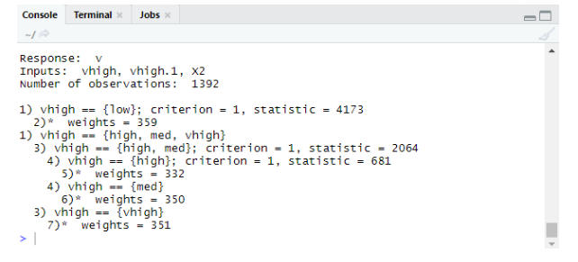
tree<-ctree(v~vhigh+vhigh.1+X2,data = train)
tree

Output:

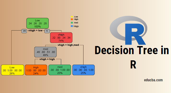
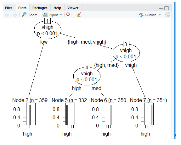
Plots Using Ctree

Prediction:

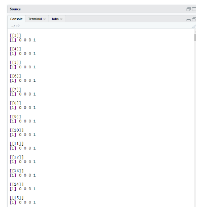
Prob generates probability on scoring,

Implementation:

predict(tree,validate,type="prob")
predict(tree,validate)

[1] vhigh vhigh vhigh vhigh vhigh vhigh vhigh vhigh vhigh vhigh vhigh

[12] vhigh vhigh vhigh vhigh vhigh vhigh vhigh vhigh vhigh vhigh vhigh

[23] vhigh vhigh vhigh vhigh vhigh vhigh vhigh vhigh vhigh vhigh vhigh

[34] vhigh vhigh vhigh vhigh vhigh vhigh vhigh vhigh vhigh vhigh vhigh

[45] vhigh vhigh vhigh vhigh vhigh vhigh vhigh vhigh vhigh vhigh vhigh

[56] vhigh vhigh vhigh vhigh vhigh vhigh vhigh vhigh vhigh vhigh vhigh

[67] vhigh vhigh vhigh vhigh vhigh vhigh vhigh vhigh vhigh vhigh vhigh

[78] vhigh vhigh vhigh high high high high high high high high

[89] high high high high high high high high high high high

[100] high  high  high  high  high  high  high  high  high  high  high

[111] high  high  high  high  high  high  high  high  high  high  high

[122] high  high  high  high  high  high  high  high  high  high  high

[133] high  high  high  high  high  high  high  high  high  high  high

[144] high  high  high  high  high  high  high  high  high  high  high

[155] high  high  high  high  high  high  high  high  high  high  high

[166] high  high  high  high  high  high  high  high  high  high  high

[177] high  high  high  high  med   med   med   med   med   med   med

[188] med   med   med   med   med   med   med   med   med   med   med

[199] med   med   med   med   med   med   med   med   med   med   med

[210] med   med   med   med   med   med   med   med   med   med   med

[221] med med med med med med med med med med med

[232] med med med med med med med med med med med

[243] med med med med med med med med med med med

[254] med   med   med   med   med   med   med   med   med   low   low

[265] low   low   low   low   low   low   low   low   low   low   low

[276] low   low   low   low   low   low   low   low   low   low   low

[287] low   low   low   low   low   low   low   low   low   low   low

[298] low   low   low   low   low   low   low   low   low   low   low

[309] low   low   low   low   low   low   low   low   low   low   low

[320] low   low   low   low   low   low   low   low   low   low   low

[331] low   low   low   low   low

Levels: high low med vhigh

Decision tree using rpart

To predict the class using rpart () function for the class method. rpart () uses the Gini index measure to split the nodes.

library(rpart)
tr<-rpart (v~vhigh+vhigh.1+X2, train)
library (rpart. plot)
rpart. plot(tr)

"

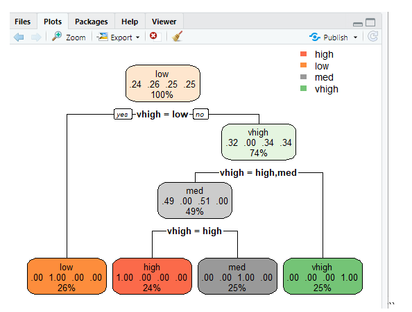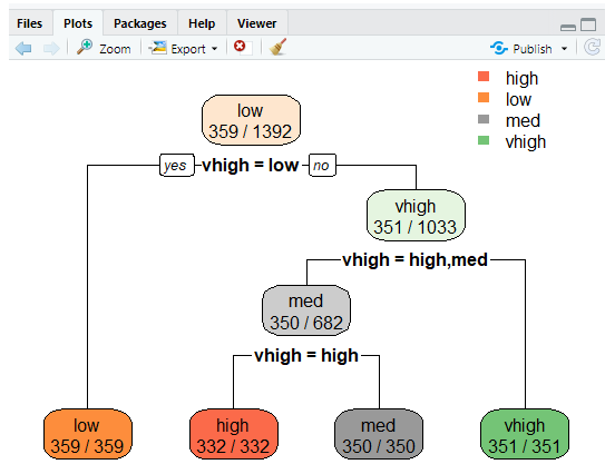
rpart.plot(tr,extra=2)

This line plots the tree and to display the probability making extra features to set 2 and the result produced is given below.

Misclassification error

The error rate prevents overfitting.

tbl<-table(predict(tree), train $v)
print(tbl)
tepre<-predict(tree,new=validate)

Output:

print(tbl)

high low med vhigh

high 332 0 0 0

low 0 359 0 0

med 0 0 350 0

vhigh 0 0 0 351

Conclusion

The decision tree is a key challenge in R and the strength of the tree is they are easy to understand and read when compared with other models. They are being popularly used in data science problems. These are the tool produces the hierarchy of decisions implemented in statistical analysis. Statistical knowledge is required to understand the logical interpretations of the Decision tree. As we have seen the decision tree is easy to understand and the results are efficient when it has fewer class labels and the other downside part of them is when there are more class labels calculations become complexed. This post makes one become proficient to build predictive and tree-based learning models.

Recommended Articles

This is a guide to Decision Tree in R. Here we discuss the introduction, how to use and implement using R language. You can also go through our other suggested articles to learn more –

1. What is a Binary Tree in Java?
2. R Programming Language
3. What is Visual Studio Code?
4. Introduction To Line Graph in R

robertsalwastion.blogspot.com

Source: https://www.educba.com/decision-tree-in-r/

Share this post